Spreadsheet Powered AI
TL;DR Multilayer perceptron that can be used to solve XOR problems only using spreadsheet formulas
How To Use the AI Sheet
Get Your Own Copy
Get Your Own Copy (Manual Method)
In case that link doesn't work, here's the main sheet (not a copy).. For obvious reasons, the main version is readonly. To play around with it, select File->Make a Copy.
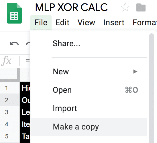
That will give you your own version of the sheet.
Iteration Issues
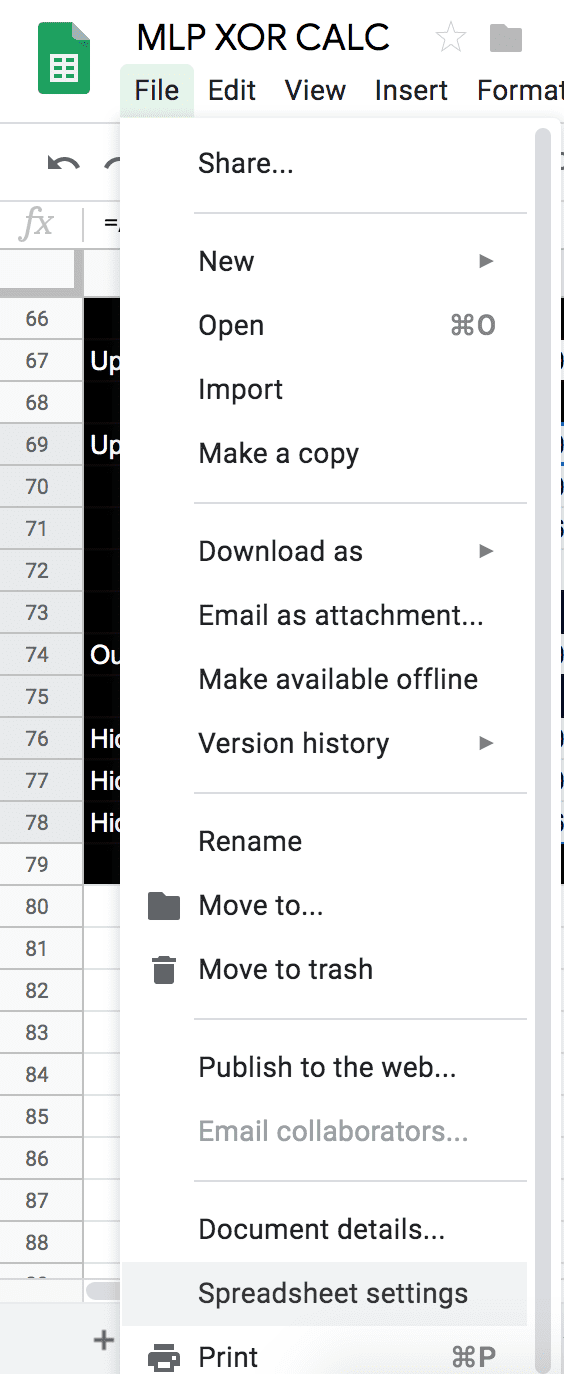
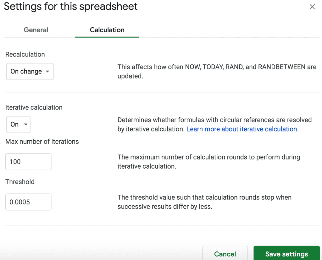
Sometimes the iterations setting for sheets won't carry over to copies. To enable this setting go to
File->Spreadsheet settings
Next, navigate to the Calculation tab and pick settings similar to these (feel free to play with max iterations, prepare for potential lag).
Running the Network
To get the network working, no ML knowledge is needed. The sheet works like a for loop, the "Current Iteration" cell D1 increments after each iteration of the network. Before incrementing, it checks the value of the "Target Iterations" cell B5. This is equivalent to the following code.
for (int current_iterations = 0; current_iterations < target_iterations; current_iterations++) {
  // run the network
}
So if you want the network to run, simply increase the value of target iterations. I would reccommend doing this in small increments (10 - 50) or the network can get out of wack. If the network does get out of wack, I've found copying cells B69:E78 then deleting and immediately pasting the cells back to be particularly effective.
I've also provided an "Update" button which simply increases the "Target Iterations" cell value by 10. You might need to enable the script on your copy of the sheet.
"Success" is when the "Current Predictions" G9:G15 match the "target result" E9:E15. At that point it has 100% accuracy with any XOR input (try moving the inputs around).
Explanation/Precursor Knowledge
If You Already Know About Neural Networks, Feel Free to Skip Ahead
Linear Separability
Data is said to be "linearly separable" if a single straight line can cleanly separate that data's features on a graph. For example, here is a graph of two distinct groups (red and blue) that are linearly separable (green line).
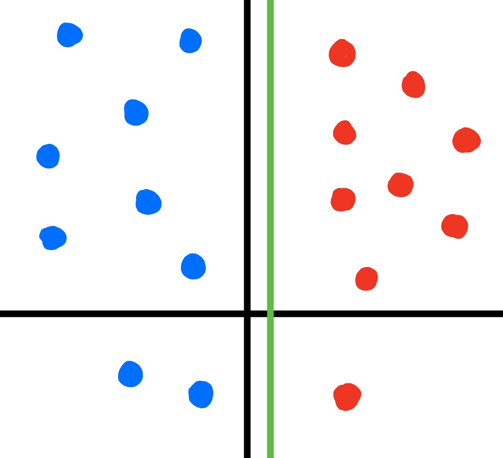
To separate data linearly, you would normally turn to an equation such as linear regression. But what if we wanted to work with data that can't be separated linearly (shown below)?
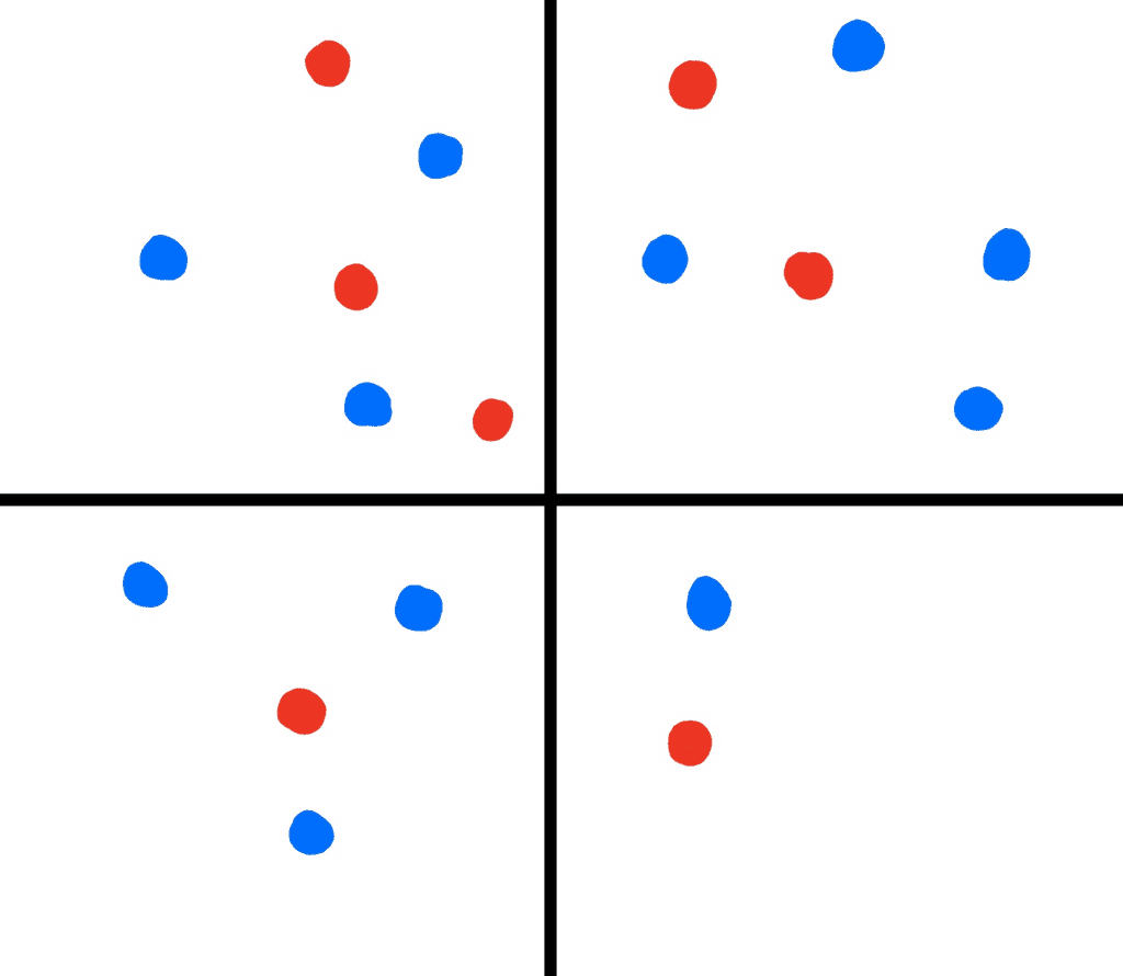
Algorithms such as SVM handle this problem by artificially adding dimensions to your data. This is done in the hope, that at higher dimensions, there exists a single line that can separate the data. But there's also another option, neural networks!
Perceptron
The simplest form of a neural network is the Perceptron (AKA the "artificial neuron"). Perceptrons take in n inputs, and give a single binary output, indicating whether the provided input was below or above a predefined threshold. Because of these principles, perceptrons are often used as binary linear separators.
But didn't we just say that we wanted to solve the separation problem for non-linear data? How can a perceptron be of use to us?
Multilayer Perceptron
Although a single perceptron can only separate data in a linear fashion, a few groups of perceptrons working together are able to accomplish the task of separating non-linear data. We refer to this collection of perceptrons working together as a MLP(multilayer perceptron). A multilayer perceptron consists of at least three layers (sets of perceptrons), the input layer, the hidden layer and and the output layer.
MLP is a supervised algorithm, which means it needs to be "told" when it correctly or incorrectly predicts something. MLP accomplishes this by having two distinct phases.
Feed-forward Stage: During this stage, the input perceptrons of the network are fed training input data. The input passes through each layer of perceptrons, eventually resulting in a single binary output that represents the "prediction" made by the network.
Back Propagation Stage: The output prediction from the feed-forward stage is compared to the expected output defined by the training set. If the predictions are correct, there is very little to be done. But if the predictions are incorrect, the network "propagates" the difference between the expected and actual results back through the network. This process gives the network a chance to "correct" the mistakes that caused the failed prediction, hopefully increasing the accuracy of subsequent runs. Usually, this is accomplished through the use of an optimization function such as the SGD (Stochastic Gradient Descent) algorithm.
XOR Problem
We need a non-linear problem that we can try and use a network to solve. To keep things simple, we'll attempt to build an "AI" that can correctly predict XOR when given a set of inputs. For those unfamiliar, XOR is a simple bitwise operator that is defined by the following truth table.
| Input Bit 0 | Input Bit 1 | Input Bit 2 | Expected Output |
|---|---|---|---|
| 1 | 0 | 0 | 1 |
| 0 | 1 | 0 | 1 |
| 0 | 0 | 1 | 1 |
| 0 | 1 | 1 | 0 |
| 1 | 1 | 0 | 0 |
| 1 | 0 | 1 | 0 |
| 1 | 1 | 1 | 0 |
If there is more than 1 bit in a row of the XOR table, the expression is false. If there exists only a single bit (as with rows 1, 2, 3), the expression is true.
Getting the Sheet Ready
To start building the spreadsheet XOR predictor, we need to first copy the XOR training set from our table (above).

B9:E15
We also need to define some stateful variables to make sure our network can persist and learn. Specifically, there variables represent the perceptrons "weights" at each layer of the network.

B74:E78
Here's the formula from one of the above cells.
IF(ISNUMBER(B69), B69, (RAND() * 2) - 1)
The weights of the perceptrons need to start out as random values in a defined range of -1 to +1. This is easily accomplished using the (RAND() * 2) - 1 formula (RAND() generates a random number from 0 - 1).
The problem arises once we need to update the weights. We don't want them to be randomly set and therefore override the progress made by our network. IF allows us to start with random values, but once cell B69 has content, the formula will use the value of that cell (instead of generating randomly).
Feed Forward Stage
Input Activation Potentials B17:E23
Next, we will begin implementing the feed-forward stage of our network. The first step is to calculate "Input Activation Potentials" by taking the dot product of each row of the training input data B9:D15 and each column of the hidden perceptron weights B76:E78.

=ARRAYFORMULA(
 IF(
 AND(current_iteration < target_iterations,
  ISNUMBER(current_iteration)),
    {
      MMULT({training_inputs, ones},
        TRANSPOSE(hidden_perceptrons)),
      ones
    },
    INDIRECT("RC", FALSE)))
The IF portion simply stops the network from looping infinitely, by checking the cell holding the current number of iterations.
IF(
AND(current_iteration < target_iterations,
 ISNUMBER(current_iteration)),
The arguments following the IF are evaluated based on the result of the branch. If...
current iterations == target iterations
we use INDIRECT("RC", FALSE), which is a comparable to using this in modern programming languages. Otherwise, we calculate the dot products using MMULT (matrix multiplication is just multiple dot products).
Hidden Layer Activators B25:E31
Next we need to calculate the activators of the hidden layer of the network. To compute the activators, we run a "activation function" on the potentials B17:E23. In practice there are many choices for your activator, in this case we will use the Sigmoid function.
Sigmoid Function
1 / (1 + exp(-x))

={
  ARRAYFORMULA(1 / ( 1 + EXP(-potentials))),
  potentials_bias
 }
Output Layer Activators B33:B39
Calculating the activations of our outputs is next. Unlike the hidden activations, we don't need to run our output potentials through the activator function. This makes calculating our output activations much easier.
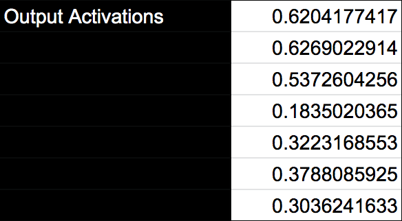
=MMULT(
  hidden_activators, TRANSPOSE(output_perceptron)
 )
Just like we did for the hidden potentials, we take the dot product of the output perceptrons B74:E74 with the "inputs" (hidden activators B25:E31) to generate the initial output of the network.
Output Binary D33:D39
We now need to take the "raw" values emitted from the output layer B33:B39 and convert them into a binary representation. This is required, because we are trying to solve a XOR problem, where only boolean values are considered valid.
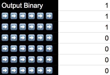
=IF(B33 < 0.5, 0, 1)
Each cell of the "Output Binary" D33:D39 checks it's partner cell in the "Output Activations" (what was calculated in the last step, cells B33:B39). If the output activation value is below 0.5, the binary result is 0. Otherwise, the binary result is 1.
Congratulations! Even though the current prediction is almost statistically guaranteed to be wrong, you can at least say a you got to the point where a prediction was made!
Backward Propagation Stage
This stage is where real "learning" takes place. Using the predictions and expected results, we calculate derivatives to adjust our weights.
Output Layer Delta F33:F39
To continue, we need to calculate the amount the output differed from the target results. This is accomplished by subtracting each target result (E9:E15) from it's corresponding output activator (B33:B39). The 2 is simply a scalar used to increase the significance of the difference.
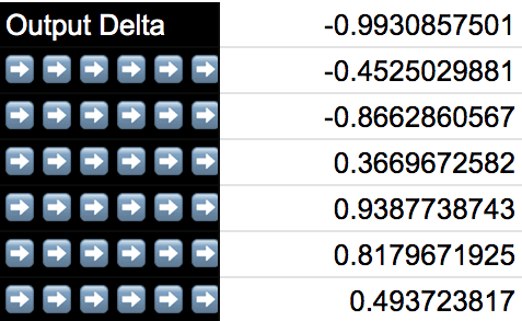
=(B33 - E9) * 2
Hidden Layer Sum B41:E47
This next step is very similar to a portion of the feed-forward stage. We're just calculating dot products between the output deltas previously calculated and the current "Output Perceptron" weight values.

=MMULT(
  output_delta, output_perceptron
 )
Hidden Layer Deltas B49:E55
Next, we determine how much the hidden layer weights should be updated. This is calculated using our hidden activators B25:E31 and the derivative of the sigmoid function (the derivative of our activator in the feed forward stage).

Derived Sigmoid Function
x * (1 - x)
=ARRAYFORMULA(
  (hidden_activators * (1 - hidden_activators)) * hidden_sum
 )
Output Change B57:E63, Output Change Average B65:E65 and Updated Output B67:E67
We want to calculate how much our output should change based on "Output Delta" F33:F39, our "Hidden Activators" B25:E31 and the "Learning Rate" B3. Due to a limitation of sheets, we have to do this in three discrete steps.
-
Output Change B57:E63
We want to calculate how much the output perceptrons should be changed. The "Output Delta" represents how much our prediction differed from the expected results. We multiply by the "Hidden Activators", because they represent the state that produced the most recent predictions.
"Learning rate" B3 is a scalar that controls how much each iteration influences the "learning" of the network. A high learning rate may sound enticing, but it introduces the possibility of overstepping a minimum and missing a convergence. Feel free to play around with learning rate, but take small steps.

=ARRAYFORMULA(
  ((output_delta * hidden_activators) * learning_rate)
 )
-
Output Change Avg B65:E65
For both clarity and practicality, it was easier to separate out the averaging of our changes into a separate step. Averaging is necessary because we are actually feeding the network 7 inputs at once B9:E15. That means we're actually dealing with 7 outputs at once, and averaging provides a way to consolidate that into a single value.

=SUM(dim0_output_change)
-
Updated Output B67:E67
Finally, subtract the calculated "Output Change Average" B65:E65 from the current values of the "Output Perceptron" B74:E74.

=ARRAYFORMULA(
  output_perceptron - output_weights_avg_change
 )
Updated Hidden B69:E72
We just updated the weights of our "Output Perceptrons" so now we need to update the weights for our "Hidden Perceptrons". Mirroring the structure used in the previous step, we use the "Hidden Deltas" B49:E55 the "Learning Rate" B3 and the "Test Input" B9:E15, to calculate how much our "Hidden Perceptrons" should change, based on the previous iteration of the network.
The TRANSPOSE({1,1,1,1,1,1,1}) represents our bias neurons, which function similarly to b in y = mx + b.

=ARRAYFORMULA(
  hidden_perceptrons - ARRAYFORMULA(
    (learning_rate * (
        MMULT(
          TRANSPOSE(hidden_delta),
          {
            training_inputs, TRANSPOSE({1,1,1,1,1,1,1})
          }
        )
      )
    )
  )
 )
Instead of the 3 distinct steps we used to calculate the Output change, we keep this condensed to a single step.
Loop
At the beginning of the explanation, we described how our weights are initialized to random values (using the RAND formula). Specifically, the IF conditional referred to a set of cells, and if those cells were empty, RAND was the fallback. Now that we have calculated valid values for the "Updated Output" and "Updated Hidden", the IF no longer evaluates the RAND branch. Instead, it proxies those "Updated" values as its own.
Output Perceptron

=IF(ISNUMBER(B67), B67, (RAND() * 2) - 1)
Hidden Perceptron

=IF(ISNUMBER(B69), B69, (RAND() * 2) - 1)
And because our "Activation Potentials" B17:E23 depend on the "Hidden Perceptrons", any updates to the "Hidden Perceptrons" force a recalculation of the "Activation Potentials". This means, as long as "Current Iteration" D1 is less than "Target Iterations" B5, the network will loop.
Idea Origin
At a previous company, I led a technical team implementing high performance neural networks on top of our core product (scale-out distributed compute platform). During this time, I quickly learned, that for most people (including upper-level management), neural networks are indistinguishable from alien technology.
It became clear, that I needed a way to explain the basic mechanics behind deep learning, without explaining the intricacies of implementing a high performance neural network. At first I tried using simple network engines written in python, but this only made sense to those who were already python programmers. But then, I had an epiphany! I realized that it might be possible to build a simple neural network, entirely with spreadsheet formulas.
